Rotten Tomatoes Review Sentiment Classification with Naive Bayes

Introduction
In this blog post, I am going to walk you through how I have implemented a Naive Bayes Classifier to classify the sentiment of Rotten Tomatoes reviews, that is to tell whether any given text review is a "Fresh" or a "Rotten".
The dataset that I used was formulated and hosted on the Kaggle platform by a user named Ulrik Thyge Pedersen. This dataset is essentially a csv file containing two columns, the first is the sentiment ("Fresh" or "Rotten") and the second is the whole review text.
Towards the end of the post, I will also showcase the experiments I have performed in the effort to improve the accuracy of the classifer, with their results that I arrived at, and the conclusions that I can draw for possible further improvement.
Alright, let's get started!
What is a Naive Bayes Classifier? (Briefly)
First of all, a Naive Bayes Classifier is also one of the many types of classifier that can be used to classify data belonging to many predefined classes. As the name already suggests, this classifier is based on the rationale behind Bayes Theorem:

That is, the chance P(H|E) that a hypothesis H holds given a set of evidence E has already happened, is proportional to the prior probability of H P(H) multiplied by the observation of the actual probability that E happens given H P(E|H).
The Bayes Theorem can be applied to update our prior belief P(H) for a certain hypothesis to a more realistic value P(H|E) by taking into consideration the factual evidence P(E|H) that has happened and fallen into the category of this hypothesis H. In our case, the hypothesis H is a review being either "Fresh" or "Rotten", and the evidence E is the set of words that review contains. The basic intuition is, from a training set of labelled reviews, we can deduce the probabilities of different words appearing in a "fresh" or a "rotten" review, and then we can apply these probabilities to other unseen reviews to classify them based on the words they contain.
The biggest limitation of this classifier is also the reason why it is called "Naive". That is, any relations between the data features are disregarded and they are all treated as being independent from each other. In the case of text classification, word ordering and grammar rules are all neglected. However, the simplification facilitates much faster training and classification, and the performance is reasonably good in practice.
Data Pre-processing
The review text data that I has got after reading directly from the input csv file is still in a state considered as "raw". That is, these texts in their original state are difficult to work with for any training and testing. Therefore, I need to perform several pre-processing steps before the data becomes usable.
Lower-casing

First off, there should be no differentiation between any letter and its upper-case counterpart. Hence, at line 2, I call the lower method on all review text strings to lower-case every letter they contain.
Punctuation Removal

Next, I remove all punctuations (such as . , : ? ! etc.) from the texts. Here, I have created two different functions for convenience. The function remove_punctuations_1 takes the review as a whole string and traverse it to remove any punctuations, whereas remove_punctuations_2 takes the already tokenized review text, i.e. a list of word strings that review contains, and removes the punctuations from each token. remove_punctuations_2 comes in handy when I may need to perform tokenization before punctuation removal, but as per final implementation, I am only making use of remove_punctuations_1, as seen on line 16 in Figure 2.
Tokenization

Then, I tokenize the review text string, that is, I split the text into words and keep only the distinct ones; All duplicate words are discarded. To perform the word by word split, I imported the re regular expression module, and called the split method, as seen on line 24.
By now, from the initially raw text strings, I have arrived at lists of distinct word strings for each of the reviews, which is ready to be used for training, validation, and final testing.
Stopword Removal

Stopword removal is an optional pre-processing step that I have implemented in the effort to improve the performance of the classifier. A stopword is basically a word that has a neutral or no special meaning, thus irrelevant when used to classify sentiment. Stopwords also appear too often and too widely, hence diminishing its effect on a review sentiment. Examples of such words can be articles like "the", "a", "an", question words like "what", "where", "when", pronouns like "I", "he", "she", etc. I will give a more in-dept discussion on the observed effect of removing stopwords later in the experimentation section.
Split the Dataset
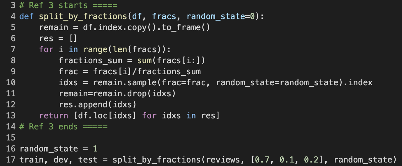
train, dev, and testOnce all text pre-processing has been completed, I continued to split the original, now clean, dataset into three subsets train, dev, and text for their respective purposes. Here, I am defining a function called split_by_fractions, which neatly splits the given dataframe up by the list of fractions provided as parameter. Lines 8 and 9 calculate the fraction frac to be splitted out with respect to the remaining fractions in the fracs list as well as the remaining samples in the dataframe. Then, lines 10 and 11 go ahead and randomly split (sample and drop) that fraction frac away from remain. These operataions repeat for as many fractions there are in the fracs list, and eventually the function will return the fractioned dataframes. split_by_fractions also takes a random_state parameter to ensure reproducibility of the split results.
Training

To calculate the priors P(fresh) and P(rotten), I first splitted the train dataframe further into train_fresh and train_rotten, which respectively has only fresh and rotten reviews. From there, the priors p_fresh and p_rotten are accordingly the ratios of len( train_fresh) and len(train_rotten) to the total len(train). Besides, I utilized the Decimal data structure to offer more floating-point accuracy over the primitive float type.
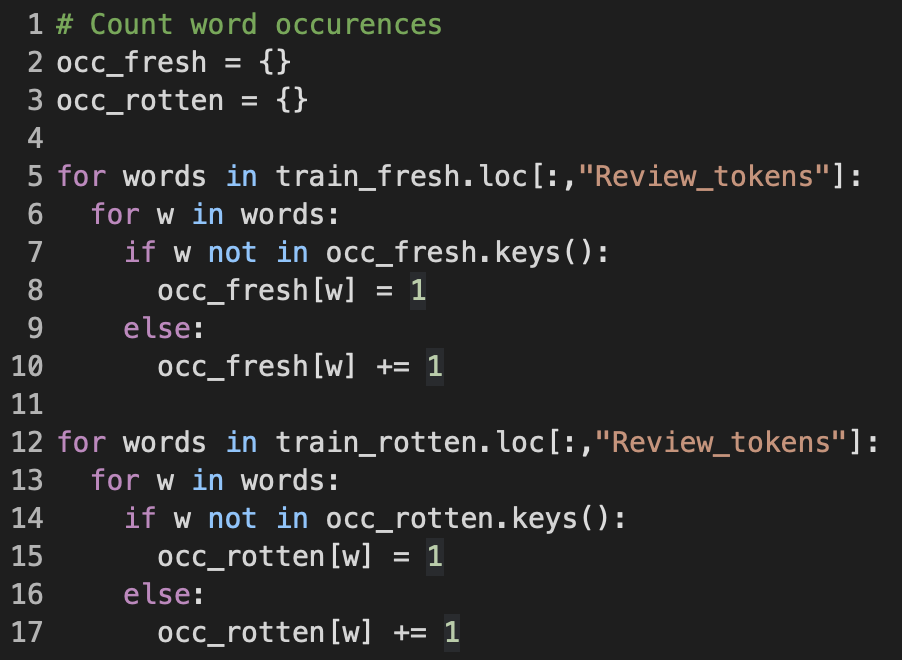
A word's occurrence is the total number of reviews in which that word appears. I decided to store the word occurrence counts as dictionaries occ_fresh and occ_rotten, whose keys are the distinct word strings, and the values are the corresponding occurrences. If a word is encountered for the first time, which means it has yet to exist in the set of dictionary keys, I initialize a new key-value pair for it and set to 1; Otherwise, I just increment the value of that word key.

With both the fresh/rotten review counts and word occurrences now available, I continued to calculate the likelihood of each word given that the review is either fresh or rotten. A word's likelihood given a review class (fresh or rotten) is equal to the ratio of that word's occurrence for that class over the total number of reviews in the class. All of the words' likelihoods are once again stored into dictionaries probs_fresh and probs_rotten, whose keys are the word strings, and the values are their likelihoods. In the calc_prob function, I iterated over occ_fresh and occ_rotten to get and pass each word's occurrence count to calc_word_likelihood. The function calc_word_likelihood then in turn calculates the likelihood of a given word based on its count and the hypothesis h. alpha is the smoothing hyper-parameter, which I will touch on in full details in a later section. The reason I separated the likelihood formula to be its own function calc_word_likelihood is because later on during the validation and test phase, it will be easier to apply smoothing to words unseen in the training set using this function.
Finally, on line 20 in Figure 8, I executed the calc_prob function with the selected alpha to produce all word likelihoods, which is what we need to perform classification.
Optimization using dev Dataset
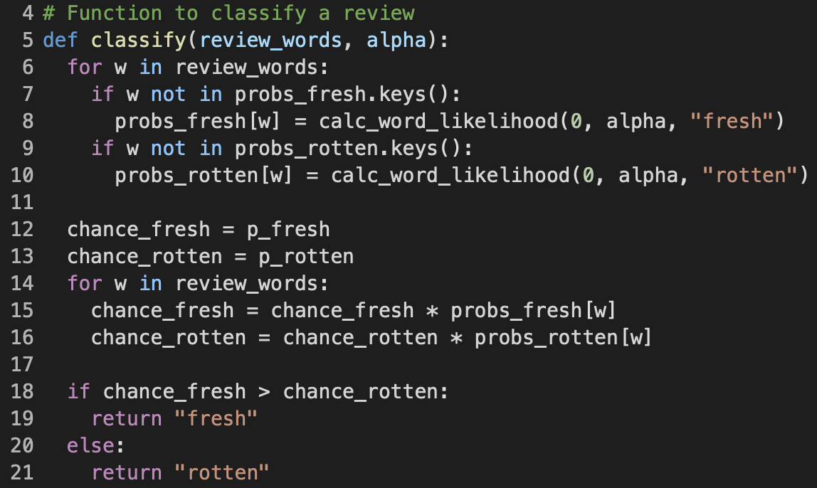
As the name suggests, the purpose of the classify function is to classify whether a given review is fresh or rotten. The function is passed the list of distinct word strings of the review, as well as the smoothing hyper-parameter alpha. In Figure 9, from lines 6 to 10, I applied smoothing to unseen words to eliminate the zero probability problem; That is, if a word does not yet exist in probs_fresh and probs_rotten, I would add it in and set its likelihood to the result of calc_word_likelihood with count of 0 and the current alpha. This also presents the reason why I separated calc_word_likelihood into its own function, as I have mentioned earlier. Next, lines 12 to 16 is where I calculated the review's chance of being fresh chance_fresh and chance of being rotten chance_rotten based on the Bayes Theorem that I have briefly discussed. And finally, at lines 18 to 21, whichever chance higher will be the class which the review is classified as.
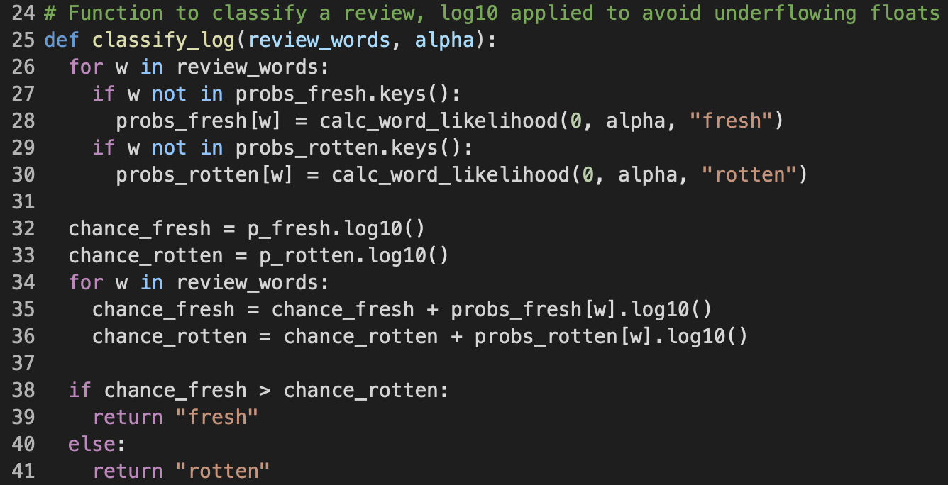
classify function but uses log probabilitiesMultiplying many less-than-one small numbers together may cause float underflowing, which means the final result can become too small to be stored in memory accurately. Therefore, to overcome such issue, I defined a second method called classify_log that performs the same task as classify, with the only difference is that it calculates chance_fresh and chance_rotten by adding up the log10's of the respective prior and word likelihoods, as seen on lines 32 to 36.
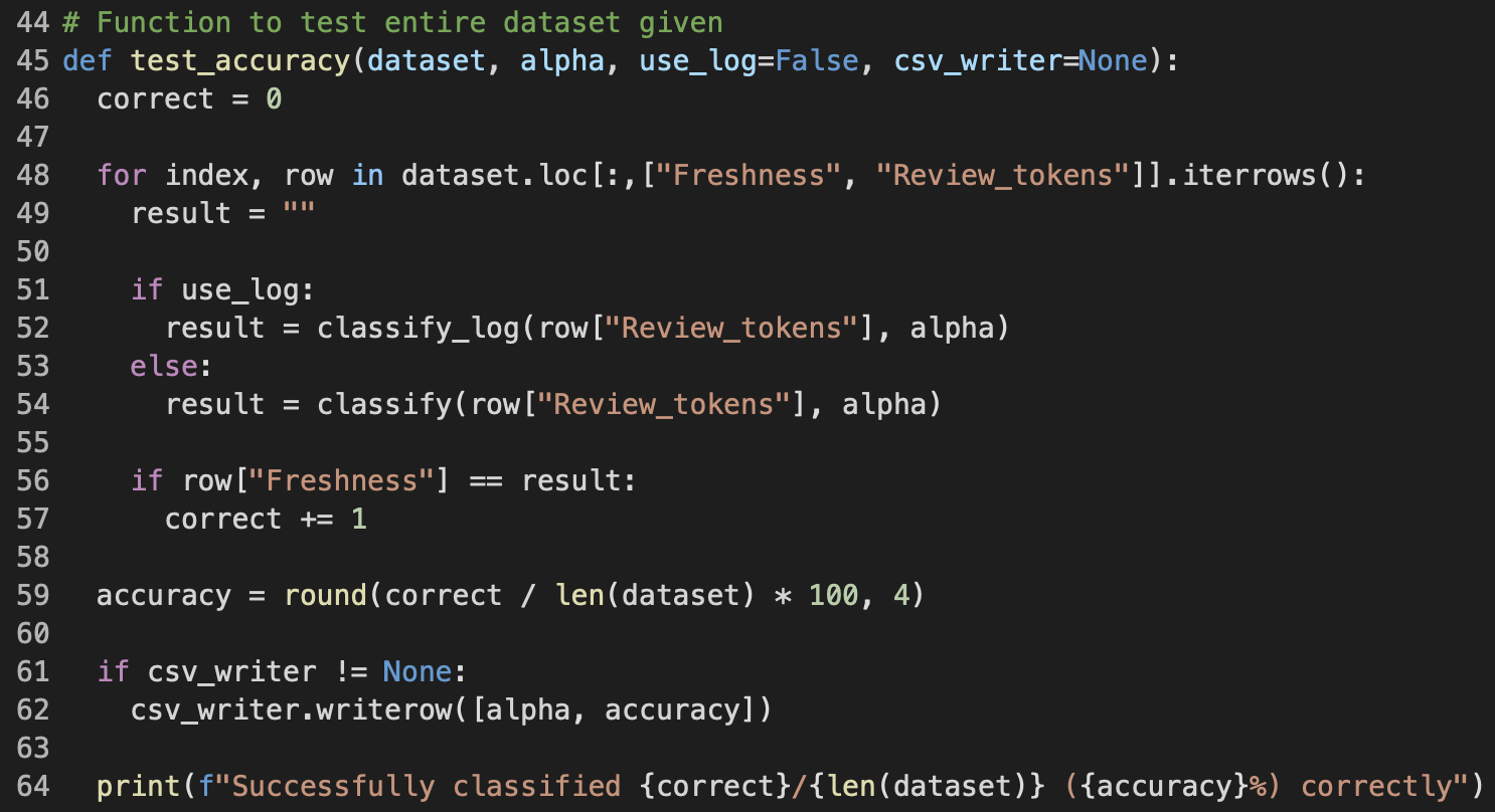
Last but not least, using the priors and word likelihoods I have derived from training, I performed the sentiment classification on each and every review in the given dataset, with alpha as my smoothing hyper-parameter of choice. The parameter use_log allows me to toggle whether I want to use classify or classify_log during testing, and based on multiple trials, I have found out that classify_log took significantly more time (around 5 times more) to finish than classify did yet the classification accuracy stayed the same; Hence, I decided to default use_log to False. The variable correct is incremented by 1 everytime a review is classified correctly, and at the end, the function will print out the number of correctly classified over the total, and the equivalent percentage representing the accuracy.
Smoothing Experiment
Earlier in the Training section, I have introduced the alpha smoothing hyper-parameter, but I have yet to discuss it in details, which is what I will be doing in this section.
The Naive Bayes Classifier suffers from an issue called "Zero Probability", which happens when a word encountered during testing has never been seen in training, hence its likelihood would be 0, causing the chances of one, or more, or even all classes to become 0, and thus the classification is undeterminable. To overcome such issue, we need to make use of "smoothing", which is basically adding a minimum value of 1 or possibly more to the occurrence count of each word, and by doing so, any words will be now considered as already seen at least once, and the zero probability will cease to happen.
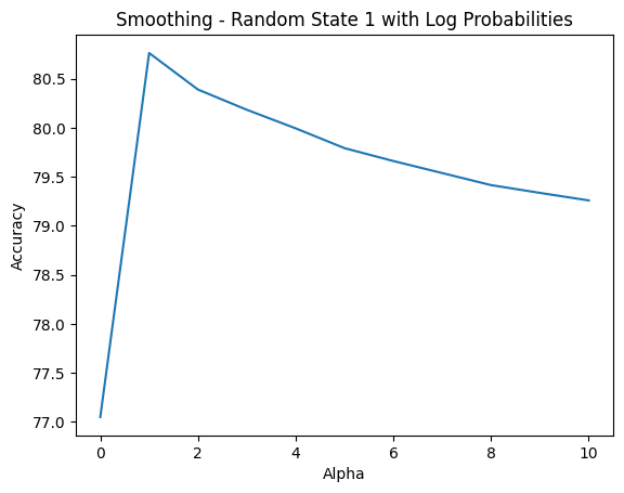
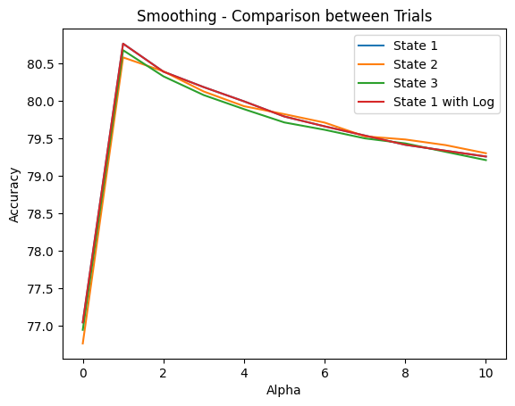
My experiment goal was to determine the smoothing hyper-parameter alpha that would yield the best classification accuracy. In addition, I had a doubt that the way I randomly splitted the original dataset into train, dev and test sub-datasets would affect the final accuracy, hence I also performed smoothing with multiple random_state to try and clarify my doubt. And the followings are visualization for the experiment data I have gathered.
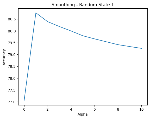
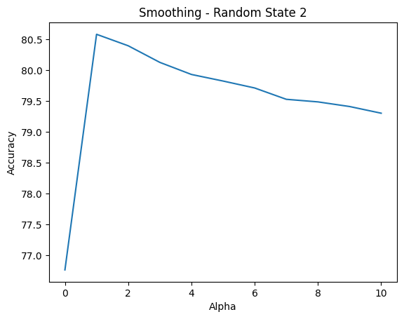
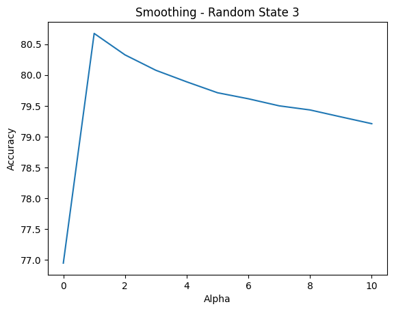
alpha ranges 0-10 and random_state ranges 1-3I could observe the same outcome, regardless of the value of random_state, is that the accuracy peaked at alpha equals to 1, and gradually decreased as I incremented alpha up to 10. To be extra guaranteed, I performed the test run on dev dataset again but now using the classify_log function for float underflow safety, and the same behavior was observed, as seen in Figure 13 below.
classify_log with random_state = 1Therefore, combining all plot lines into a same coordinate system as in Figure 14 below, I can confidently conclude that the value of 1 is the best choice for the smoothing hyper-parameter alpha, and the way I performed dataset split did not interfere with the achieved classification accuracy as the outcomes stayed consistent throughout different random_state's.
Stopword Removal Experiment
Stopword removal is another technique that can help improve the performance of the classifier by removing words that are neutral and irrelevant when it comes to deciding the sentiment of a review containing such word. Without performing any stopword removal yet, I observed that the following words in Figure 15 were the most predominant in either the fresh or rotten class.
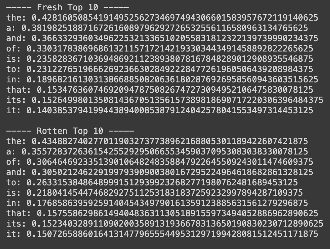
And I think, looking at these words, you can agree with me that they are all neutral, common words, and given that a review contains any of these words, we will still have a hard time classifying it as fresh or rotten. Therefore, we should try to filter out all words unnecessary for classification, and possibly the accuracy will improve.
The nltk package, which is widely known and used for nature language processing in machine learning, offers a list of common stopwords. After removing the stopwords from nltk's list, I got an accuracy of 80.5896 %, which is actually lower than the accuracy without stopword removal of 80.7625 %. Furthermore, the followings are the new top 10's.
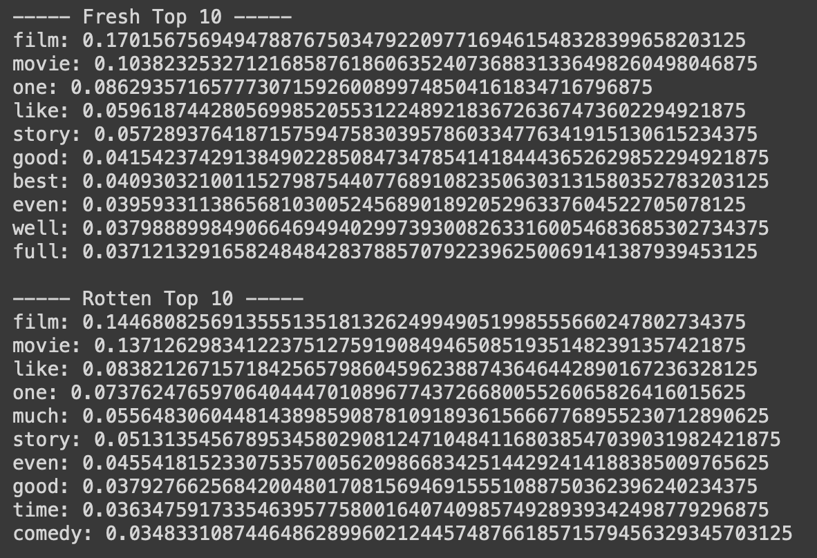
nltk's stopwordsFrom the way it seemed, I had definitely removed the unwanted stopwords. However, similar neutral words across the two classes like "film", "movie", "story" were still predominant, and also the accuracy actually dropped by a small fraction. That led me to believe that I should craft my own list of stopwords for better result, because optimal stopwords are different for different datasets; There exists no single universal list of stopwords. And that was what I did.

At line 19 in Figure 17, my custom list of stopwords starts with the common neutral words. And as the top 10 words for fresh and rotten classes changed under the effect of these stopwords, I handpicked the next list of words to be added into stop_words. I stopped after 14 rounds, and the graph in Figure 18 below is what I got in terms of accuracy reactions towards the stopwords added in.
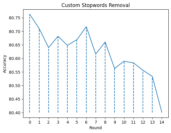
stop_words listMy heuristics for considering a word as a stopword were that the meaning of the word was neutral or irrelevant and/or the word likelihood appeared to be the same for both classes. My expectations were that eventually I would arrive at the top 10 words that were remarkably different between the two classes, and the accuracy would increase by a little or a lot. As a result, my first expectation holds as seen in Figure 19 below; On the contrary, the accuracy ended up being lower than without performing stopword removal (round 0).
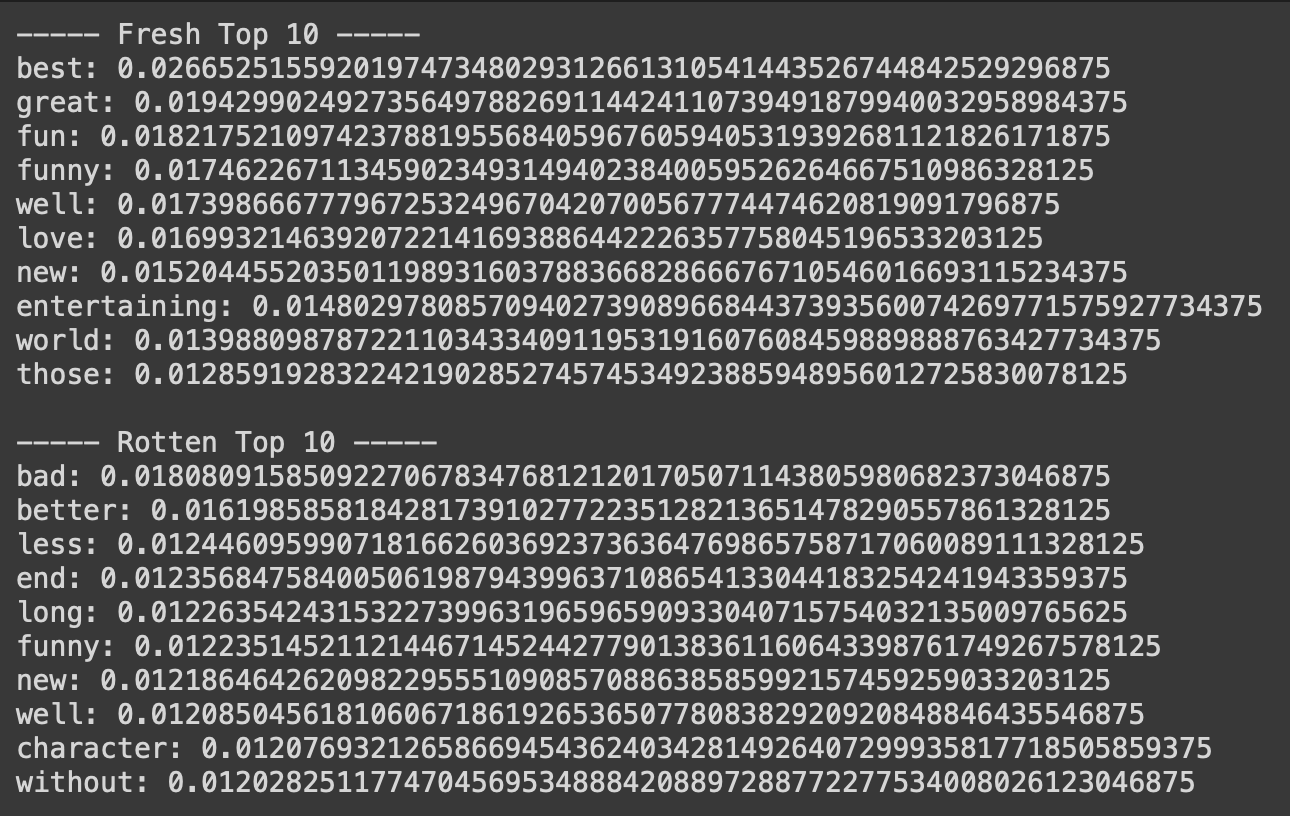
Possible explanations for this result can be that my stopword-choosing heuristics are not 100% correct, or that even though some words are neutral in meaning, fresh or rotten review givers tended to use them more than their counterpart did, causing these seemingly unnecessary words to become somewhat influential in classification. Nonetheless, I have successfully picked out the two lists of words that really matter for a fresh or rotten review.
Final Accuracy
After performing the two experiments, I have decided to set smoothing alpha to 1 and not perform stopword removal. The final accuracy that I achieved on the test dataset was:

which is highly consistent with what I have achieved using the dev dataset.
For future improvements, I can fine-tune my stopword list for hopefully a marginally better accuracy, given the fact that 80% accuracy is already considered a really good achievement. Moreover, I can introduce stemming and lemmatization to compress related words into a single representative word, thus reduce the correlation between separate words, which goes against the independence assumption in Naive Bayes.
Last words: My full code implementation and code references can be found here.
