Image Classification with PyTorch
Introduction
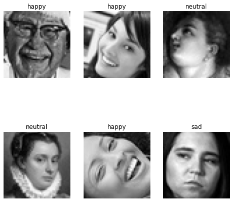
In this blog post, I will show you how I have implemented an image classifer using the PyTorch machine learning library. Under the hood, the image classifier is a convolutional neural network, which is a version of the plain multi-layer perceptron specialized to work best with learning and classifying images. The dataset I will be using is the facial emotion expression images created by a user named Samaneh Eslamifar on the Kaggle platform.
My end goal, within the limited time allowed, is to successfully build an image classifier based on this tutorial from PyTorch and experiment to improve its classification performance as best as possible. And before we jump into the nitty-gritty of implememtations, you can find my jupyter notebook, as well as line-by-line references, here.
Alright, let's get down to business!
Download the Dataset from Kaggle
I implemented the image classifier in a jupyter notebook run on Google Colab. Therefore, I need to download the facial expression dataset into the remote host machine before I can start working with it.
Kaggle provides a simple mechanism to download any datasets, whether from a competition or just a hosted dataset, by installing their Python module kaggle and place the kaggle.json API key file, which can be downloaded from your Kaggle account webpage, under the path ~/.kaggle on the machine. Once everything is set up, the dataset can be downloaded with one command kaggle datasets download [dataset name]. Following is the full codes:
        ! pip install kaggle
        ! mkdir ~/.kaggle
        ! cp /content/drive/MyDrive/kaggle.json ~/.kaggle/
        ! chmod 600 ~/.kaggle/kaggle.json
        ! kaggle datasets download samaneheslamifar/facial-emotion-expressions
        ! unzip facial-emotion-expressions.zip
In jupyter notebook, preceeding a code line with an exclamation ! means we want to run this line as a Linux terminal command.
Here, I am downloading the whole samaneheslamifar/facial-emotion-expressions dataset and saving it locally on the remote runtime. The downloaded dataset sometimes may still be compressed as a zip file, so we need the final command to unzip it.
Label the Data
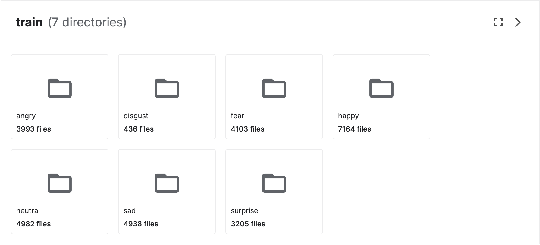
In order for any neural network training and testing to be performed, we need a rich dataset AND for all data samples in the set to be labelled. Our facial expression dataset here is indeed of high quality, but unfortunately, the image data samples are yet to be labelled in a machine-learnable manner, but just categorized into different directories. Therefore, it is our job to now produce the appropriate data labels.
First off, there are 7 different facial emotions into which the images are categorized: angry, disgust, fear, happy, neutral, sad, surprise. For a machine to more easily make sense of this difference emotion classes, we map each of them to an integer starting from 0, as below:
        label_map = {
            "angry": 0,
            "disgust": 1,
            "fear": 2,
            "happy": 3,
            "neutral": 4,
            "sad": 5,
            "surprise": 6
        }
We then want to match each image to the integer associated with the class that image is assigned into. In our case, we will match the image file name with the integer, and write everything into two CSV files called train_labels.csv and test_labels.csv; By that way, we can later on easily read these CSV files to load the images and their labels into Dataset and DataLoader objects that the neural network can directly access and benefit from their optimized underlying data structure. Below is the full implementation of this process.
        train_csv = open("train_labels.csv", "w")
        train_writer = csv.writer(train_csv)
        test_csv = open("test_labels.csv", "w")
        test_writer = csv.writer(test_csv)

        train_root = "/content/images/train"
        for label in sorted(os.listdir(train_root)):
          for img in sorted(os.listdir(os.path.join(train_root, label))):
            train_writer.writerow([os.path.join(label, img), label_map[label]])

        test_root = "/content/images/validation"
        for label in sorted(os.listdir(test_root)):
          for img in sorted(os.listdir(os.path.join(test_root, label))):
            test_writer.writerow([os.path.join(label, img), label_map[label]])
As you can see, we have to traverse the directory structure to read every image file name, and match it with a label integer depending on which sub-directory like angry, fear, disgust, etc. that image is located in.
And our result CSV files will have their contents looking some like this, with first column for image name, second column for label integer, and every row is an image data sample:
        angry/10052.jpg,0
        angry/10065.jpg,0
        angry/10079.jpg,0
        angry/10095.jpg,0
        angry/10121.jpg,0
        ...
Load into Dataset and DataLoader objects
Perfect! Now we have got all the data locally accessible and labelling out of the way, the last thing to do before we can get to building our neural network is to load the data in as tensors, which the network will directly train and test on, from the external dataset.
As our facial emotion expression dataset is a custom one and not pre-packed with PyTorch like the MNIST datasets, we need to create our according custom Dataset class, as well as DataLoader instances that the network can use to iterate over the data samples while training and testing.
Any custom dataset class must extend from the Dataset class and define three methods: __init__, __len__, and __getitem__
        class FacialExpDataset(Dataset):
          def __init__(self, labels_csv, img_dir, transform=None, target_transform=None):
            self.img_labels = pd.read_csv(labels_csv)
            self.img_dir = img_dir
            self.transform = transform
            self.target_transform = target_transform

          def __len__(self):
            return len(self.img_labels)

          def __getitem__(self, idx):
            img_path = os.path.join(self.img_dir, self.img_labels.iloc[idx, 0])
            image = read_image(img_path).float()
            label = self.img_labels.iloc[idx, 1]
            if self.transform:
              image = self.transform(image)
            if self.target_transform:
              label = self.target_transform(label)
            return image, label
__init__ is the constructor of the custom dataset class. Here, we want our custom FacialExpDataset to take in as attributes: the path to all images (img_dir), the path to the label CSV file (labels_csv), and transform and target_transform for any extra transformation operations respectively on the images and the labels.
__len__ will return the total number of samples in the dataset based on the total number of labels there are.
__getitem__ defines how a sample from the dataset should be returned. In this case, we will return a 2-element tuple of the full image file path and the integer label ranging from 0 to 6 as there are seven image classes.
With the dataset custom class now fully defined, we can go ahead and create Dataset instances for our image data, as below:
        one_hot_transform = Lambda(lambda y: torch.zeros(
            7, dtype=torch.float).scatter_(dim=0, index=torch.tensor(y), value=1))
        train_data = FacialExpDataset("/content/train_labels.csv", train_root,
                                        target_transform=one_hot_transform)
        test_data = FacialExpDataset("/content/test_labels.csv", test_root,
                                        target_transform=one_hot_transform)
We need to perform a transformation operation on the labels called one-hot encoding, hence we use a Lambda function called one_hot_transform. One-hot encoding will turn the integer label into a 7-dimensional vector, with 0's in all dimensions except for a 1 at the index equal to that label value. The reason we need to perform such transformation is because our neural network will not classify by outputting a single integer indicating which class an image belongs to; Instead, it will output a 7-dimensional vector of probability values which show how confident the network thinks that the image belongs to the class with integer label same as the value index.
Finally, to iterate over train_data and test_data, we need DataLoader instances:
        batch_size = 3
        train_loader = DataLoader(train_data, batch_size, shuffle=True)
        test_loader = DataLoader(test_data, batch_size, shuffle=True)
Normally in PyTorch, single data samples are batched together to perform batch training and testing, thus here, we set the batch_size to 3 so that each batch for loss calculation and optimization step will consist of feeding 3 data images through the network. train_loader and test_loader are respectively set to be the iterators for train_data and test_data Datasets. Besides, we set the option shuffle to True to ensure images are randomly fetched and fed into the network for better training and testing.
Build the Neural Networks
We will build two neural networks. The first network is similar to the one implemented in this PyTorch tutorial. The second network is a custom one in which we will add more convolutional layers to see how this change affects the classification accuracy.
The first neural network, as I call itOriginalNeuralNet, is defined as below:
        class OriginalNeuralNet(nn.Module):
          def __init__(self):
            super().__init__()
            self.conv1 = nn.Conv2d(1, o_conv1_cn, 5)
            self.pool = nn.MaxPool2d(2, 2)
            self.conv2 = nn.Conv2d(o_conv1_cn, o_conv2_cn, 5)
            self.fc1 = nn.Linear(o_fc1_in, o_fc1_out)
            self.fc2 = nn.Linear(o_fc1_out, o_fc2_out)
            self.fc3 = nn.Linear(o_fc2_out, 7)

          def forward(self, x):
            x = self.pool(F.relu(self.conv1(x)))
            x = self.pool(F.relu(self.conv2(x)))
            x = torch.flatten(x, 1)
            x = F.relu(self.fc1(x))
            x = F.relu(self.fc2(x))
            x = self.fc3(x)
            return x
OriginalNeuralNet has two convolutional layers conv1 and conv2, one max-pooling layer pool and three dense layers fc1, fc2, and fc3. The feed-forward flow will be: conv1 → max pool 2x2 → conv2 → fc1 → fc2 → fc3.
The second neural network, which I call ConvNeuralNet, is defined as below:
        class ConvNeuralNet(nn.Module):
          def __init__(self):
            super().__init__()
            self.conv1 = nn.Conv2d(1, conv1_cn, 3)
            self.conv2 = nn.Conv2d(conv1_cn, conv2_cn, 3)
            self.conv3 = nn.Conv2d(conv2_cn, conv3_cn, 3)
            self.conv4 = nn.Conv2d(conv3_cn, conv4_cn, 3)
            self.pool = nn.MaxPool2d(2, 2)
            self.fc1 = nn.Linear(fc1_in, fc1_out)
            self.fc2 = nn.Linear(fc1_out, fc2_out)
            self.fc3 = nn.Linear(fc2_out, 7)

          def forward(self, x):
            x = F.relu(self.conv1(x))
            x = self.pool(F.relu(self.conv2(x)))
            x = F.relu(self.conv3(x))
            x = self.pool(F.relu(self.conv4(x)))
            x = torch.flatten(x, 1)
            x = F.relu(self.fc1(x))
            x = F.relu(self.fc2(x))
            x = self.fc3(x)
            return x
The differences, compared to OriginalNeuralNet, are that there are now two extra convolutional layers conv3 and conv4, the kernel size of all convolutional layers are set to 3 by 3, and the feed-forward flow is now: conv1 → conv2 → max pool 2x2 → conv3 → conv4 → max pool 2x2 → fc1 → fc2 → fc3. My hope when building ConvNeuralNet like such is that adding more convolution layers into the network will in return improve the its accuracy. Nonetheless, we will need to perform network training and test to find out, which is what we will do next!
Train and Test the Neural Networks
As for computing resources, I used Google Colab's Premium GPUs for much higher performance thus saving time.
For the loss function and optimizer, I chose to use Cross Entropy and Stochastic Gradient Descent:
        loss_func = nn.CrossEntropyLoss()
        def optimizer(net):
          return optim.SGD(net.parameters(), lr=learning_rate)
The first two hyper-parameters I needed to set was the total number of epochs and the learning rate. I chose to go with 7 epochs, as after many runs I observed that the network's accuracy peaked at around epoch 7 or 8 without any further improvement. And for the learning rate, I set it to 0.001 as this is a common value for this hyper-parameter.
The following are the train loop function, test loop function, and the train_test function to actually execute the training and testing:
        def train(data_loader, net):
          total_batch_num = len(data_loader)
          running_loss = 0.0
          optim = optimizer(net)
          for i, (images, labels) in enumerate(data_loader):
            images = images.to(device)
            labels = labels.to(device)

            optim.zero_grad()

            outputs = net(images)
            loss = loss_func(outputs, labels)

            loss.backward()

            optim.step()

            running_loss += loss.item()
            if (i+1) % 2000 == 0:
              print(f'[{i+1}/{total_batch_num} batches]: avg loss = {running_loss/2000:.3f}')
              running_loss = 0.0
The train loop is a typical one where for each data batch, the parameter gradients are cleared, new outputs and loss are calculated, backpropagation is performed on the loss, and optimizier take a step to update all parameters accordingly.
        def test(data_loader, net):
          correct = 0
          total = 0
          with torch.no_grad():
            for images, labels in data_loader:
              images = images.to(device)
              labels = labels.to(device)
              outputs = net(images)
              _, predicted = torch.max(outputs, 1)
              _, truth = torch.max(labels, 1)
              total += labels.size(0)
              correct += (predicted == truth).sum().item()
          return 100 * correct // total
The test loop iterates through the whole test_set, runs the trained network on each batch, and calculates the precentage of correctly classifed images.
        def train_test(net, csv_file, csv_writer, csv_row):
          total_train_time = 0.0
          for epoch in range(num_epochs):
            print(f"\nEpoch {epoch+1}\n-------------------------------")
            start = time.time()
            train(train_loader, net)
            train_time = time.time() - start
            total_train_time += train_time

            train_res = test(train_loader, net)
            test_res = test(test_loader, net)
            csv_row.append(train_res)
            csv_row.append(test_res)
            print(f"Traing Set Accuracy: {train_res} %")
            print(f"Test Set Accuracy: {test_res} %")

          print(f"\n----- Final Accuracy Verification -----")
          final_res = test(test_loader, net)
          csv_row.append(final_res)
          csv_row.append(total_train_time)
          print(f"Accuracy: {final_res}")
The train_test function calls to the train and test loops to train the network and test it right after each epoch. At the end of all epochs, it calls the test loop one last time to verify the final accuracy achieved. Here, we also record the total time it takes to train the network.
Experimentations
The idea is that I will try to increase the number of learnable parameters gradually up to the point that the network shows signs of overfitting. Signs of overfitting can be that the training time is significantly larger, or the classification accuracy per epoch on the train set still increases close up to 100%, but that of the test set starts to decline. The network-associated hyper-parameters I will be experimenting with are the convolutional output channels and the inputs and outputs of the fully-connected layers.
Once I have reached at the so-called "optimal" set of hyper-parameters for both of the original and my custom neural networks, I will compare their classification performance as per epoch, which will then prove that adding more convolutional layers into the network will improve its accuracy or not.
First, we will discuss the experimentation with the OriginalNeuralNet.
OriginalNeuralNet training performance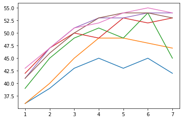
OriginalNeuralNet testing performance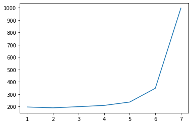
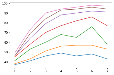
OriginalNeuralNet training time takenThe three graphs above summarize the training performance, testing performance, and training time taken for the OriginalNeuralNet over 7 different groups of learnable parameters. To increase the number of parameters from one group to the next, I multiplied each of the numbers of channels of the convolutional layers by 2. The numbers of channels for all convolutional layers are powers of 2.
As the network becomes more complex with more parameters, the training performance (Figure a) rises close to the accuracy of 100%. In the meanwhile, the respective testing performance (Figure b) also rises, and we can observe that the few top lines converge to the accuracy limit of this network, which means around 54% to 55% accuracy is the best that this network can achieve given its architecture. How can we tell this? By Figure c. The training time spikes after I increased the number of parameters from group 6 to group 7, whereas the testing performance only improves slightly as depicted by the pink line in Figure b. This means any attempts to introduce even more parameters will only overfit the network, as it has nearly perfectly classified the training set.
Next, let's take a look at the experimentation with my custom ConvNeuralNet.
ConvNeuralNet training performance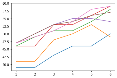
ConvNeuralNet testing performance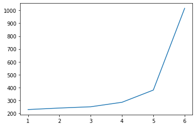
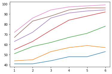
ConvNeuralNet training time takenThe next three graphs here summarize the training performance, testing performance, and training time taken for the ConvNeuralNet over 6 different groups of learnable parameters. The way I increased the parameters from one group to the next is the same as what I did for the OriginalNeuralNet.
The same pattern we can observe immediately is that the more parameters the network has, the better it performs, and as the training performance (Figure d) approaches close to 100%, testing performance (Figure e) also converges to an accuracy of approximately 57% to 60%. The same situation applies for the training time taken (Figure f), as in it rises steeply and signifies that the network is close to overfitting. The difference in how our custom network behaves compared to the original one is that an increase in parameters will give us a noticeable improvement in the starting performances of each group, as shown in Figure d that one line is completely over on top of another and none of them intercepts. So, this raises the question: Does adding more convolutional layers improve the network's performance?
The answer is Yes, as we take a look at the graph below comparing the best versions only of the orignal and custom network.
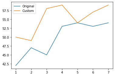
OriginalNeuralNet versus ConvNeuralNetNow that's what I am talking about! Judging from Figure g, we can conclude the neural network architecture does impose an impact on the performance of the network, and in the sense that the more convolutional layers a network has, the more accurate it classifies. The x axis represents the 7 epochs, and the y axis is the network accuracy for the test set. Figure g clearly shows that ConvNeuralNet performs better than OriginalNeuralNet in every epoch. Therefore, my future intention is to design a network with more convolutional layers, and push the network size like I did in the experiments above until I can reach a satisfactory accuracy.
Technical Challenges
The most remarkable challenge I would say is the limitation on computing resources.
The more I tried to push extra parameters into the network, the more computing intensive it was to train it, which sometimes could result in a total crash due to memory depletion.

Therefore, it will be more preferable to have access to abundant resources for unconstrained network training and testing.
