Kaggle Competition: Titanic - Machine Learning from Disaster

Introduction

If you are like me, a software engineer who is picking up an interest on the field of data science, and is making his first baby steps in machine learning, then look no further because I know just the right place for you to start: Kaggle Competitions. Not knowing where to apply your newly learnt machine learning knowledge and try out some models? Worry not because Kaggle has got you covered! The Kaggle platform hosts many machine learning competitions, in each of which you are provided with the dataset, as well as a web-based Jupyter notebook environment, so you can jump straight into the fun part of implementation without doing any tedious setups.

In this blog post, I will show you how I have followed the tutorial for the Titanic - Machine Learning from Disaster competition where participants attempt to predict the survivability of passengers based on various attributes such as age, passenger class, sex, etc. All participants have a limited number of submissions per day, and they compete against each other by achieving the best accuracy in the fewest number of submissions. And instead of Kaggle notebook, I will be using Google Colab for my implementation. Alright, let's get started!

Data Exploration

First off, we need to import the necessary packages, and in this case (but also most cases), they are numpy and pandas for respectively numerical and data manipulation.

        import numpy as np
        import pandas as pd

Next, we will need to perform some data exploration before we can deduce any intuition or patterns. The dataset is provided as two files called "train.csv" and "test.csv", and as the names suggest, the first is for training our machine learning model, whereas the latter is for testing its accuracy. We use pandas to load the files in as DataFrame, which is essentially a two-dimensional table with objects as rows and their attributes as columns.

        train_data = pd.read_csv("/content/train.csv")
        train_data.head()

        test_data = pd.read_csv("/content/test.csv")
        test_data.head()

As the outputs above present, we can see what attributes each passenger possesses. And in the train_data, we can see that each passenger has already been classified as survived or not according to the "Survived" column, which serves as the ground truth label necessary for model training.

Our First Intuition

Given the data and the context of the Titanic disaster, one of our first intuitive predictions can be that all the female passengers survived while the male did not; Because as part of the evacuation protocol, women and children were given prority over men, thus their chance of survival would be much greater. We can test this assumption using the train_data.

        women = train_data.loc[train_data.Sex == 'female']["Survived"]
        rate_women = sum(women)/len(women)
        print("% of women who survived:", rate_women)
        

        men = train_data.loc[train_data.Sex == 'male']["Survived"]
        rate_men = sum(men)/len(men)
        print("% of men who survived:", rate_men)
        

We use the loc operation on the data frames to extract a list of values that satisfy the row and column conditions in the square-bracket subscripts. In this case, the row condition was either the "Sex" was all "male" or "female", and we took the whole "Survived" as the column condition. Dividing the sum of elements, which were 1 for those who survived and 0 otherwise, by the length of the whole list, which also equals the total number of male or female, gives us percentages of male or female that survived. And much to our favor, the percentage of women surviving was significantly higher than that of men. Therefore, we can go forth and generate a submission based solely on passengers' gender.

        gender_prediction = np.where(test_data.Sex == "female", 1, 0)
        gender_output = pd.DataFrame({"PassengerId": test_data.PassengerId, "Survived": gender_prediction})
        gender_output.to_csv("gender_submission.csv", index=False)
        

Here, we make use of the where operation offered by numpy to quickly create a list of 0's and 1's, in that all female passengers will be classified as survived and the opposite for all male. Lastly, we combine the list of passenger ids with gender_prediction to create a new data frame that will be our first submission to the competition. And guess how much did we score?

Over 70% accurate? Not bad for a first try and for the fact that we have just used only one single attribute in the data! Obviously, however, there are a lot of rooms for improvement here. We have to consider a few more factors, like: What if the wealthy passengers of higher class had received evacuation privilege? And, what if passengers had evacuated in family and relative groups instead of as each individual, which makes a lot more sense? That is why the tutorial has led us to now consider four attributes "PClass" (Passenger class), "Sex" (Gender), "SibSp" (Number of siblings and/or spouses), and "Parch" (Number of parents and/or children) of each passenger to see how these can determine the outcome.

Our First Actual Machine Learning Model!

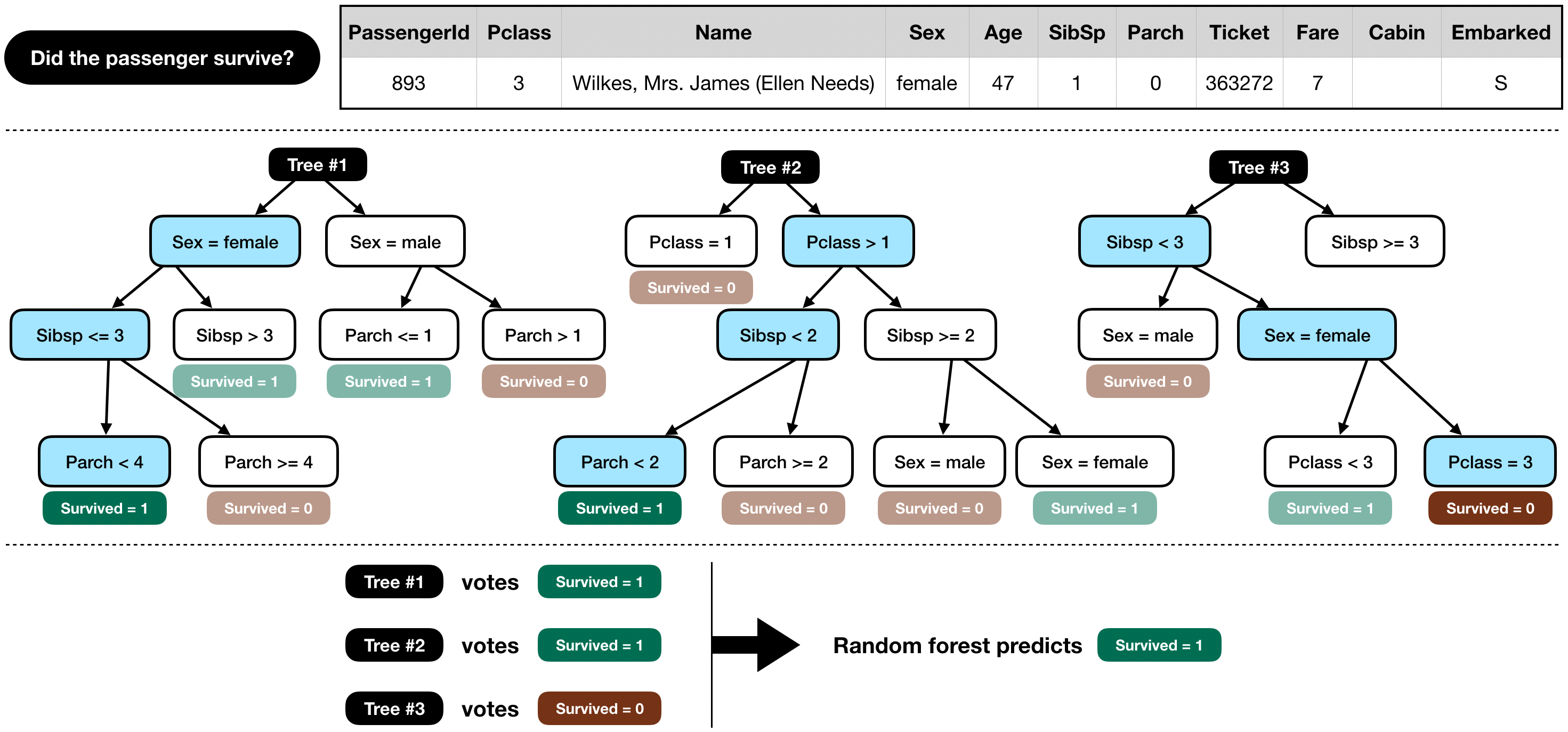
The tutorial introduces us to a pre-defined machine learning model called RandomForestClassifier, which is part of the well-known and widely-used ML Python library scikit-learn. RandomForestClassifier is an ensemble type of model, which means the model arrives at its prediction based on the "votes" of multiple constituent classifier algorithms; In this case, each constituent is a Decision Tree, hence many of them will form up a Forest. Once all Trees have concluded, the classification with the most votes i.e. has been concluded with the most, will be the final outcome.

So, first thing we need to do is to select and prepare the pieces of data that we want to later feed into the model for training.

        from sklearn.ensemble import RandomForestClassifier

        y = train_data["Survived"]
        
        features = ["Pclass", "Sex", "SibSp", "Parch"]
        
        X = pd.get_dummies(train_data[features])
        X_test = pd.get_dummies(test_data[features])
        
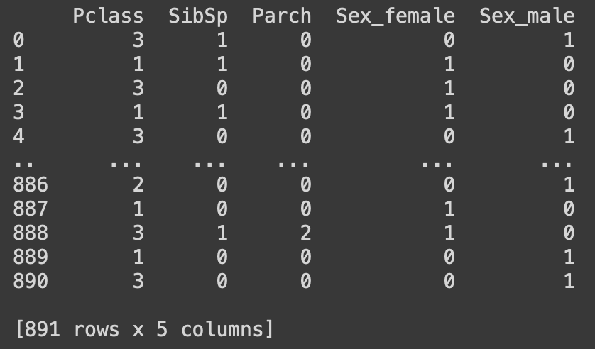
        print(X)
        

The variable y is set to hold the entire "Survived" column from train_data; Later, we will use y as the target to try and fit our model to. features is the list of columns we will extract from train_data and test_data, the rest will be ignored. According to pandas documentation, what the get_dummies function does is "convert categorical variable into dummy/indicator variables"; And as in the above image, the attribute "Sex" was categorical, so it was transformed into two separate columns "Sex_female" and "Sex_male", both of which were indicators for a passenger's gender. Performing these prepping steps on both train_data and test_data respectively gave us the two data frames X and X_test. Now we are ready for the training and predicting.

        model = RandomForestClassifier(n_estimators=100, max_depth=5, random_state=1)
        model.fit(X, y)
        predictions = model.predict(X_test)
        
        output = pd.DataFrame({'PassengerId': test_data.PassengerId, 'Survived': predictions})
        output.to_csv('rfc_submission.csv', index=False)
        

For the parameters of the RandomForestClassifier model, we set n_estimators to 100, which means there would be a total of 100 Decision Trees, and the max_depth of each is set to 5 so every Tree will conclude after at most 5 decisions. The training actually happens when we call fit on the model and pass in X and y. Once training finishes, we let the model predict given X_test. The final results are again formatted into a data frame and outputed as a csv file to be submitted to the competition. How well will we do this time? Fingers crossed!

Hooray! We make a .1 improvement in accuracy! Now this may seem like such a trivial gain, but when it comes to machine learning in practice, any increments even the slightest means that we are going in the right direction. All that is left to do now is to keep finding ways to improve, and that is the spirit I love about machine learning!

P.S. You can view my Jupyter notebook on my GitHub repository here, or directly on your browser here